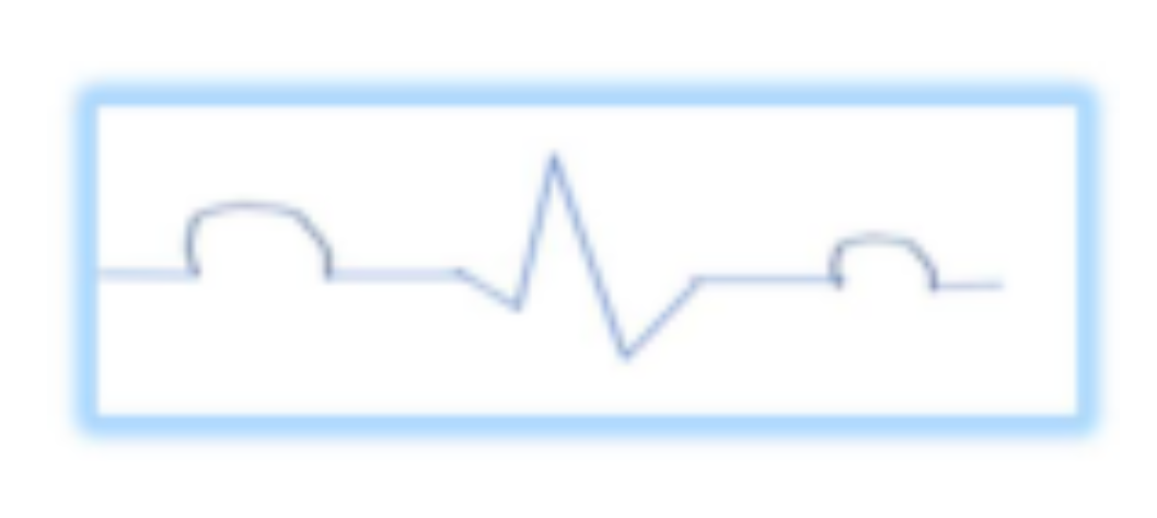
It is always said that do whatever your heart says and makes you happy, but do you know how your heart works and is your heart healthy or unhealthy? We have always seen a few zigzag lines (Fig. 1) on a machine kept near a patient in movies that shows the health condition of the patient.
Fig 1: Zigzag lines and electrocardiogram
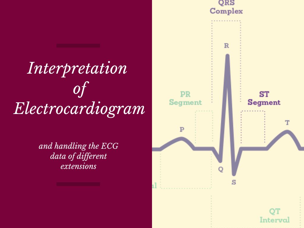
Do you wonder how it is done? These lines help to understand the heart rhythm and electrical activity of the heart. This type of graph is known as ECG (Electrocardiogram) and the machine is an ECG recording machine. The ECG machine stores information about the heart electronically, which is used by doctors. Let’s understand the interpretation of ECG data in detail. Fig 2 shows how a doctor sees the curves and interprets them.
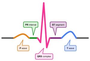
Fig 2: Electrical Activity of the Heart (fig source link)
Few leads/sets of electrodes are placed on the skin of a person and record the electrical activity of the heart. There are 10 electrodes present in a standard ECG. The 12 leads are I, II, III, AVL (augmented vector left), AVR (augmented vector right), AVF (augmented vector foot), V1, V2, V3, V4, V5 and V6. The electrodes are responsible for conducting signals that cause the heart to contract. ECG tracing specifically shows the depolarization wave during each heartbeat.
Some of the steps include:
The signal waveform files can be accessed using the WFDB (waveform database) package. There are a lot of extensions in which the signal data is stored. WFDB file formats include header (WFDB header file format), annot (WFDB annotation file formats), signal (WFDB signal file formats) and webcal (WFDB calibration file format). For all signals, the standard set of 12 leads (I, II, III, AVL [augmented vector left], AVR [augmented vector right], AVF [augmented vector foot], V1, V2, V3, V4, V5 and V6.) with reference electrodes on the right arm was stored. The electrodes capture the signal at 12 leads.
The signal data can be stored in .dat files and .header files. Files with .dat extension contain data but the data can be loaded when the information about data is present.
Loading the file with data extension is a tough process as these files may contain text, images, video, audio, etc. File with textual data can be loaded in any text editor. Files with videos can be loaded in any media player.
In case of ECG signals, the data was loaded using the WFDB package. But if you have to work on Fourier transform then your data should be in integer form not in waveform. The conversion of the .dat file to .csv is necessary for doing Fourier transform of signals. Let’s study this in depth.
The conversion of .dat files to .csv files was a tremendous process for me. As the .dat did not open in any of the editors except in the WFDB package. The dat file was loaded in the WFDB package using wfdb.rdrecord and then plotted using wfdb.plot_wfdb. As wfdb returns an object it was unable to print. This was the mistake I made in the process and I lost time.
As a result, the second approach was used. Different ways were tried to load a dat file that can return an array or something but not an object. After some attempts numpy library serves as a savior and np.fromfile(‘file_name.dat’,dtype=float) returns an array. The array is stored in a csv file by using np.savetxt(“name.csv”, y, delimiter=”,”) and then the Fourier transform is applied.